Visualizing layers of the Inception model
In this tutorial, we will visualize the various features detected by different channels of the deep layers of the convolutional neural network model called Inception. In this machine learning problem, instead of fixing the input/output and learning the weights, we fix the weights and learn what input maximizes the output.
[Link to the Jupyter Notebook]
Last time we went over loading the pre-trained Inception5h model and running it on our own input images in excrutiating level of detail. This time we focus on visualizing the features that the different channels of various layers have been trained to detect. If you are already comfortable with tensorflow and neural networks, DeepDreaming with TensorFlow is a great read, otherwise, here is a less technical version of that tutorial with a couple of lengthy detours. Lets go ahead and load the model:
In [1]:
import tensorflow as tf
import numpy as np
import PIL.Image
from IPython.display import clear_output, Image, displaymodel_fn = 'tensorflow_inception_graph.pb'
mygraph = tf.Graph()
sess = tf.InteractiveSession(graph=mygraph)with tf.gfile.FastGFile(model_fn, 'rb') as f:
graph_def = tf.GraphDef()
graph_def.ParseFromString(f.read())t_input = tf.placeholder(np.float32, name='input')
tf.import_graph_def(graph_def, {'input':t_input})layers = [op.name for op in mygraph.get_operations() if op.type=='Conv2D' and 'import/' in op.name]
print('Number of Conv2D layers: ', len(layers))
Out:
Number of Conv2D layers: 59
Andrew Ng has an excellent course on Convolutional Neural Networks on Coursera. If you just want to know what convolutional layers are, the second video of the course goes through an example of a convolution operation starting around 01:20. Basically, you can think of covering a part of your input image with a filter, the result of that being your output (both your input image and the filter are nothing but numbers, you just have to multiply one by the other in a particular way to get the "output" number), then sliding the filter to a different part of the image. Repeat until you've dragged the filter all over the - say, two-dimensional - input, and produced the two-dimensional output. Naturally, the filter should be smaller than your input image - it could be 3x3, 5x5, etc. The thing about filters is that different filters detect different things. These things could be a vertical edge in the input, a horizontal line, a wavy squiggle at 45 degrees, etc. Roughly speaking, if the input contains what the filter is looking for, the output is maximized. As a soon-to-be-former-physicist, I like convolutional NNs because they make use of the translational invariance property: if you are interested in whether the input image contains a cat, you don't care where the cat is located on the image. That's why filters that slide over the entire image come in handy!
Continuing my hand-waving guide to deep learning, lets see what the computer is actually learning in this scenario. When you start showing it images, at first the computer has no idea what kind of features to look for, so initially the filters are just matrices populated with random numbers (this should start to sound familiar). In an image classification problem, the network classifies each image (input) as belonging to a particular category (output). While training, the computer compares its output to the correct answers, and adjusts the trainable variables W to get its output(s) closer to those correct values.
In convolutional layers, W are the filters: for a 3x3 filter, there is a total of nine values the computer will learn and later will use to classify the new input images it has not seen before. In a given layer, there are often multiple filters of the same size that are detecting different features (e.g., one for vertical and one for horizontal lines, etc). Lets see what kind of convolutional layers is the Inception network made up of:
In [2]:
import re
for i in range(len(layers)):layers[i] = re.search('import/(.+?)/conv',layers[i]).group(1)
print(layers)
Out:
['conv2d0_pre_relu', 'conv2d1_pre_relu', 'conv2d2_pre_relu', 'mixed3a_1x1_pre_relu', 'mixed3a_3x3_bottleneck_pre_relu', 'mixed3a_3x3_pre_relu', 'mixed3a_5x5_bottleneck_pre_relu', 'mixed3a_5x5_pre_relu', 'mixed3a_pool_reduce_pre_relu', 'mixed3b_1x1_pre_relu', 'mixed3b_3x3_bottleneck_pre_relu', 'mixed3b_3x3_pre_relu', 'mixed3b_5x5_bottleneck_pre_relu', 'mixed3b_5x5_pre_relu', 'mixed3b_pool_reduce_pre_relu', 'mixed4a_1x1_pre_relu', 'mixed4a_3x3_bottleneck_pre_relu', 'mixed4a_3x3_pre_relu', 'mixed4a_5x5_bottleneck_pre_relu', 'mixed4a_5x5_pre_relu', 'mixed4a_pool_reduce_pre_relu', 'mixed4b_1x1_pre_relu', 'mixed4b_3x3_bottleneck_pre_relu', 'mixed4b_3x3_pre_relu', 'mixed4b_5x5_bottleneck_pre_relu', 'mixed4b_5x5_pre_relu', 'mixed4b_pool_reduce_pre_relu', 'mixed4c_1x1_pre_relu', 'mixed4c_3x3_bottleneck_pre_relu', 'mixed4c_3x3_pre_relu', 'mixed4c_5x5_bottleneck_pre_relu', 'mixed4c_5x5_pre_relu', 'mixed4c_pool_reduce_pre_relu', 'mixed4d_1x1_pre_relu', 'mixed4d_3x3_bottleneck_pre_relu', 'mixed4d_3x3_pre_relu', 'mixed4d_5x5_bottleneck_pre_relu', 'mixed4d_5x5_pre_relu', 'mixed4d_pool_reduce_pre_relu', 'mixed4e_1x1_pre_relu', 'mixed4e_3x3_bottleneck_pre_relu', 'mixed4e_3x3_pre_relu', 'mixed4e_5x5_bottleneck_pre_relu', 'mixed4e_5x5_pre_relu', 'mixed4e_pool_reduce_pre_relu', 'mixed5a_1x1_pre_relu', 'mixed5a_3x3_bottleneck_pre_relu', 'mixed5a_3x3_pre_relu', 'mixed5a_5x5_bottleneck_pre_relu', 'mixed5a_5x5_pre_relu', 'mixed5a_pool_reduce_pre_relu', 'mixed5b_1x1_pre_relu', 'mixed5b_3x3_bottleneck_pre_relu', 'mixed5b_3x3_pre_relu', 'mixed5b_5x5_bottleneck_pre_relu', 'mixed5b_5x5_pre_relu', 'mixed5b_pool_reduce_pre_relu', 'head0_bottleneck_pre_relu', 'head1_bottleneck_pre_relu']
Lets look at the first layer and check what are the filter dimensions and how many filters are there. For the latter, we look at the last number in the shape of the tensor, corresponding to the output of the first layer:
In [3]:
print(mygraph.get_tensor_by_name('import/conv2d0_pre_relu:0').get_shape())
Out:
(?, ?, ?, 64)
The first three positions in the tensor's shape are question marks because in tensorflow, tensors are symbolic and only obtain numerical values when evaluated inside a tensorflow session. The first three values will depend on what is fed into the network: the batch size (number of images), then we have two dimensions for the ouput of each filter, and finally the number of filters in this layer, 64, which has no dependence on the input.
Now we know there are 64 filters in the layer called conv2d0_pre_relu; what about the size of the filters? We can look at the size of the weight matrix for this layer. To get weights and biases from a pre-trained network that we read from a .pb file, we look at the constant nodes of the graph:
In [4]:
weight_nodes = [n for n in graph_def.node if n.op=="Const"]
weight_names = [n.name for n in weight_nodes]
print(weight_names[0:10])
weights = dict(zip(weight_names, weight_nodes))
Out:
['conv2d0_w', 'conv2d0_b', 'conv2d1_w', 'conv2d1_b', 'conv2d2_w', 'conv2d2_b', 'mixed3a_1x1_w', 'mixed3a_1x1_b', 'mixed3a_3x3_bottleneck_w', 'mixed3a_3x3_bottleneck_b']
The nodes called conv2d0_w and conv2d0_b contain the pre-trained weights and biases, respectively, for the first (zeroth, if we want to use the same naming convention) layer. These are NodeDef objects that contain various information, but lets just check the size of the filters for the first few convolutional layers:
In [5]:
def get_weight_size(layer) :
return [d.size for d in weights[layer].attr['value'].tensor.tensor_shape.dim]
print(get_weight_size('conv2d0_w'))
print(get_weight_size('conv2d1_w'))
print(get_weight_size('conv2d2_w'))
Out:
[7, 7, 3, 64]
[1, 1, 64, 64]
[3, 3, 64, 192]
Evidently, the filter size of the first convolutional layer is 7x7x3. 3 comes from there being three channels for RGB (colored) images, and 64, as we already established, is the total number of filters (which becomes the number of channels for the next layer, hence the 64 in 1x1x64, etc).
Inception 5h seems to be a realization of the so-called GoogLeNet network, whose architecture you can see in Fig. 3 of the Going deeper with convolutions paper. Starting with layer 3, multiple filter sizes are used at the same layer, hence the mixed in the layer names: mixed3a_1x1_pre_relu, mixed3a_3x3_pre_relu, mixed3a_5x5_pre_relu etc. This allows the Inception model to detect features at different lengthscales. Speaking of features, it is time to look at some of those!
Visualizing layers of the Inception model
In the previous tutorial we talked about how the computer learns the appropriate values of W (trainable parameters - weights and biases) during training. When using a pre-trained model, you already have values for W, but there is something else that we can learn. As I explained last time, when training a neural network, we feed input X into the first layer, where it gets multiplied by the weights W1 to produce output Z1. Z1 (or, when using an activation function such as ReLU, A1 = ReLU(Z1)), then serves as input for the second layer, and this just goes on until we get the final output Z. We compute the appropriate weights Wi from minimizing the difference between Z and the correct output Y.
Lets say the training has finished, and Wi are fixed. In CNNs, each channel of each convolutional layer is associated with a particular filter, trained to detect a particular feature / set of features. To vizualize the features detected by a chosen channel, we can see what kind of input is needed to maximize the output of that channel. Mathematically, this problem is very similar to the one we were solving during training of the CNN, except that instead of minimizing the difference between Z and Y, we are now maximizing some output Zi for the ith layer, and the variables that we are solving for are X instead of W.
In [6]:
def display_output(a, screen=True, name=None, save=False) :
#Using the raw output of a layer for visualization purposes doesn't work very well,#so we normalize it to get the right range of values#Here I use the constants from the 'DeepDreaming with TensorFlow' tutorial
a = (a-a.mean())/max(a.std(), 1e-4)*0.1 + 0.5
a = np.uint8(np.clip(a, 0, 1)*255)
img = PIL.Image.fromarray(a)
#display image on the screen
if screen == True:display(img)
#save the rendered image to a file
if save == True and name != None:img.save("%s.jpg"%name)
''' Arguments:
layer: name of the layer
channel: number of the channel whose output is to be maximized
img0: the initial input image, that will be modified to max the channel's output
save_file = True if the final image is to be saved as a jpeg file
iter_n, step: parameters for the gradient descent
'''
def render_channel(layer, channel, img0, save_file=False, iter_n=30, step=1.0) :
#output of the channel :
t_output = mygraph.get_tensor_by_name("import/%s:0"%layer)[:,:,:,channel]#mean value of the output (this is what we want to be maximized) :
t_mean = tf.reduce_mean(t_output)#get the derivative of the [mean] output with respect to the input
t_grad = tf.gradients(t_mean, t_input)[0]img = img0.copy()
for i in range(iter_n):g = sess.run(t_grad, {t_input:np.array(img)[np.newaxis,:]})
g /= g.std()+1e-8
#update the input image (delta = gradient * step)
img += g[0,:]*stepdisplay_output(img, name="%s_%s"%(layer, channel), save=save_file)
''' Visualize all the channels present in the layer. Try 'mixed4b_1x1_pre_relu'
if you are on the market for pretty, yet understated psychedelic wallpaper!
'''
def visualize_layer(layer) :
#number of channels in the layer :
channels = int(mygraph.get_tensor_by_name("import/%s:0"%layer).get_shape()[-1])for c in range(channels):
img_noise = np.random.uniform(size=(224,224,3)) + 100.0
print('Layer ',layer,' channel ', c)
render_channel(layer, c, img_noise)
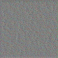
# Let's visualize channel 97 of layer mixed4a_1x1_pre_relu :
img = np.random.uniform(size=(224,224,3)) + 100.0
render_channel('mixed4a_1x1_pre_relu',97,img)
Out:

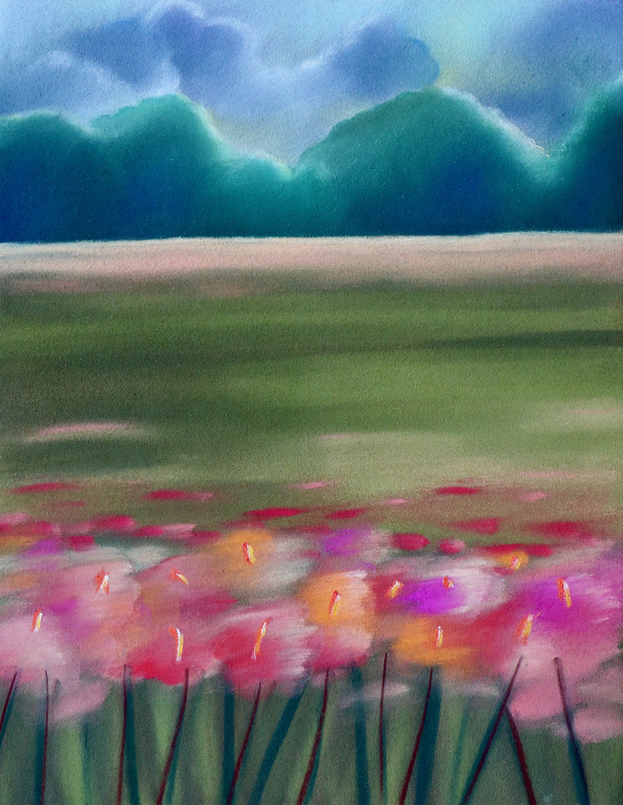
As the table below demonstrates, the closer the layer is to the input, the more microscopic are the attributes it had been trained to detect, and on the contrary, the deeper the layer - the more abstract the features. First we detect, basically, things like edges, then edges start to form patterns, patterns eventually form objects, etc. One can imagine filters trained to detect eyes (mixed4c_pool_reduce_pre_relu channel 0), parts of buildings (mixed4c_pool_reduce_pre_reluchannel 61), and flowers (mixed4d_3x3_bottleneck_pre_relu channel 139). You should, however, keep in mind that many of these are going to be merely our brains' attempts to interpret what we are seeing as something that makes sense to us. For instance, as much as the output of mixed4b_pool_reduce_pre_relu channel 45 may resemble creepy human faces, the classification categories that GoogLeNet was trained to detect do not, in fact, include people.


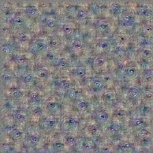


Another thing that is evident is that features keep getting repeated on our derived "input" images. This makes sense given the nature of the convolutional layers: namely, the way that the filter slides over the image.
In [7]:
sess.close()

Inception: getting started
The simplest guide to using the Inception model that you'll ever see
I have been playing around with generating images using the Inception5h model that has been trained on around a million images from the 1000 Imagenet categories. When I first started this, being relatively new to tensorflow, I wished there was a simple guide, explaining exactly what each line of the code was doing. So if you find yourself in this situation, if you are new to tensorflow, Python, and/or neural networks or machine learning in general, this tutorial is for you!
It is a little annoying that Squarespace won't let me simply paste the HTML version of my original Jupyter notebook into the blog post, but here is a link to it (try this one if GitHub fails to render the Ipynb file).
The simplest guide to using the Inception model that you'll ever see
I have been playing around with generating images using the Inception5h model that has been trained on around a million images from the 1000 Imagenet categories. There is no shortage of tutorials on how to use pre-trained neural networks, but when I first started this, being relatively new to tensorflow, I wished there was a simple guide, explaining exactly what each line of the code was doing. So if you find yourself in this situation, if you are new to tensorflow, Python, and/or neural networks or machine learning in general, this tutorial is for you :)
Lets get started! If you have not done so already, get the Anaconda Python distribution and install tensorflow. I like the Spyder IDE that comes with Anaconda, so let's go ahead, open it, and start coding:
In [1]:
import tensorflow as tf
import numpy as np
To use a pre-trained model, the first thing you'll need is to get your hands on one. You can download a copy of the Google-trained Inception model for image recognition here. Unzip and place the file called tensorflow_inception_graph.pb in the same directory as your Python code. If you want a more technical version of what I am doing in this post, I would recommend the DeepDreaming with TensorFlow tutorial, where much of the code here is coming from.
The .pb file contains the model's graph. TensorFlow is a symbolic library, with tensors corresponding to data structures, and graphs representing the computations to be performed on them.
If you are already familiar with the basic idea behind artificial neural networks, you will want to skip this and go straight to the next line of Python code
If your math is a bit rusty, you don't need to worry about graphs and tensors for the moment, just think of them as equations written in terms of variables. When you were a kid, you may have been given an equation like
6 − 2*w = 0
and asked to find the value of w that satisfies this equality. That is sort of what neural networks are about. Training one is like finding the right w, except that your equation does not have a solution, and you are just trying to find the value of w (a.k.a. weights and biases) that will get the right side of your equation close enough to zero for your purposes.
Supervised learning and Image Classification
That equation thing from the paragraph above does not sound very useful, does it. That is because so far we have omitted a crucial part of machine learning: the data itself. Say you have a bunch of pictures of cats and dogs and you want your computer to learn to recognize what's on them. To the computer, each of those pictures is nothing more than a bunch of numbers. Since you only want it to be able to distinguish cats from dogs, you really only need two options for an asnwer: say, 0 for a dog, 1 for a cat (I am a cat person, can you tell).
Mathematically, what you need is a function that will take an image X (remember, X is nothing but a bunch of numbers), and output either 0 or 1. But how do you construct the right function? You don't. Your computer will do it for you.
In reality, the function we just described, probably does not exist. But we could come up with one that gives the right answer very often, perhaps 99% of the time or more - and truth be told, not even a human can distinguish a teacup pomeranian from a persian kitten, a baby seal, or a superior alien species, every single time.

I don't know who you are, but I love you already!
For a computer to learn what cats and dogs look like, it will have to - you guessed it - look at a lot of cats and dogs. The function you want your computer to come up with at the end will be parametrized by a bunch of variables W (this W is kind of like the w we saw above, but now it is bold and capitalized to emphasize that it is, in fact, a bunch of variables). First, your computer will use some random initial values of W, put your images through the resulting function, and compare the value it gets, Z, to the correct answer you'll provide it with, Y. Now, you had your input images X, the correct 0 or 1 answers for each image Y, and you've got your computer's guesses Z. By the way, this is called supervised learning because you supplied the correct answers for the training images. The value of Z depends on W. What you now want is to minimize the difference between Z and Y for all of your training images. In other words, once you sum over the training data, you have some equation like this
Difference between Y and Z (a function of W) = 0
and you want the computer to find the values of W that will get the right side as close to zero as you want. Once done, you can feed your computer new images it has not seen before, and the hope is that it will classify them correctly as cats and/or dogs.
So the neural network is basically a very complicated function with lots of parameters W and that is what is contained in the file tensorflow_inception_graph.pb.
In [2]:
model_fn = 'tensorflow_inception_graph.pb' #yep, that's the name of the file with the graph
First, you want to create a Graph object. A Graph contains a set of tf.Operation objects, which represent units of computation; and tf.Tensor objects, which represent the units of data that flow between operations. 1
In [3]:
mygraph = tf.Graph()
We could have skipped this, in which case a default graph would have been created once you start a tensorflow session. We'll want to be able to refer to it though, and having to say tf.get_default_graph every time is just cumbersome.
Now let's go ahead and load the saved model into our computation graph:
In [4]:
# Start a tensorflow session with the Graph mygraph
sess = tf.InteractiveSession(graph=mygraph)
In [5]:
with tf.gfile.FastGFile(model_fn, 'rb') as f:# "f" is how we will refer to the 'tensorflow_inception_graph.pb' file from now on
graph_def = tf.GraphDef() # GraphDef object is what we get when we save a Graph object
    # Now you want to read the data from the file into the GraphDef object
    graph_def.ParseFromString(f.read())
# You'll need to define an entry point into your model: the placeholder for the input X that will be fed into it
t_input = tf.placeholder(np.float32, name='input')
tf.import_graph_def(graph_def, {'input':t_input}) # This will import the graph from graph_def into mygraph
Inception is a deep convolutional neural network meaning it has many layers. Roughly speaking, it means that you take the input X, multiply it by some variable W1, call the result Z1, put it through something called an activation function (don't worry about what this is, neural networks just work better this way than with simply feeding Z1 directly into the next step) and obtain A1. For the next layer, take A1 as the new input, multiply by W2 to get Z2, feed it to a (possibly different) activation function and get A2. Repeat until you reach the last layer, and call your last result output. In the cat vs. dog classifier discussed above, the final output will be 0 or 1 (you could also have it be a real number between 0 and 1, like 0.7 - in case the computer wants to say that it is 70% sure it is looking at a cat, but there's a 30% chance it is a dog after all).
By now, the structure of the neural network is buried inside our Graph mygraph along with all the weights W. Let's dig it up and see what it looks like:
In [6]:
layers = [op.name for op in mygraph.get_operations() if op.type=='Conv2D' and 'import/' in op.name]
Layers is now a list containing (surprise!) names of layers. It actually only includes the names of the convolutional layers of the Inception network, but those are the more interesting ones when it comes to computer vision anyway. How many are there?
In [7]:
print('Number of Conv2D layers: ', len(layers))
Out:
Number of Conv2D layers: 59
That is a deep neural network indeed! As we will see in the next tutorial, there is a certain hierarchy to what kind of features are detected at which depth. The more basic features, such as lines, are detected by the layers closest to the input image. The deeper layers can detect patterns that those lines form, and if you go yet deeper, you'll be detecting objects. The neat thing is that you can literally see, on an image, what each layer of the network is checking for, but we'll get to that next time.
Now lets use the image of the white pomeranian puppy above and see what Inception will think of it. First, lets prepare the JPEG to be fed into the tensorflow graph:
In [8]:
import PIL.Image
image = PIL.Image.open("pommy.jpg")
image_array = np.array(image)[np.newaxis, :, :, 0:3]
We have added an additional (dummy) axis, because the model is configured to process multiple images at a time while training (these groups of images are called batches). Then we've got width, height, and the three RGB values - these roughly correspond to the amount of Red, Green, and Blue in the color for each pixel. (For a greyscale image, we would only need to keep one value per pixel - the intensity.)
Now we'll feed image_array into the input layer, and compute the output. Here is the code to do that:
In [9]:
output_tensor = sess.graph.get_tensor_by_name('import/output2:0')
prediction = sess.run(output_tensor, {'input:0': image_array})
Prediction now holds the probabilities (put differently, degree of faith) the Inception model estimates for the image to contain one of the 1000 image categories (plus an additional null category for when the image does not seem to match anything Inception was trained to recognize). I expected the prediction array to have dimensions of (1, 1001), but interestingly, that is not the case:
In [10]:
print(prediction.shape)
Out:
(42, 1008)
Unfortunately, this version of the Inception model is not very well documented, but from what I was able to find online, the seven extra categories are there for obscure historical reasons and are to be ignored. The 42 is a little more interesting. First of all, why is it 42? Is that a reference to the Hitchhiker's Guide to the Galaxy? (It probably is.) In any case, I am not sure how to interpret these columns, but one guess I have is that the model might be detecting different parts of the image as an object, and that's why there are multiple answers for each image category. We can play around with checking if this is the case later, but for now lets take the maximum value of each row:
In [11]:
prediction = prediction.max(axis=0)
In the same ZIP where we got our .pb file, there is a text file with strings corresponding to the 1000 + 1 category labels. Lets read it into an array, and then output the top five choices for what is depicted in our input image:
In [12]:
labels = 'imagenet_comp_graph_label_strings.txt'
lines = open(labels).readlines()top_pred = prediction.argsort()[-5:][::-1]
for i in range(5):print(i+1, ' ', lines[top_pred[i]].strip('\n'), ' ', int(prediction[top_pred[i]]*100), '% \n')
Out:
1 Persian cat 97 %
2 Angora 18 %
3 Pekinese 7 %
4 Maltese dog 6 %
5 Shih-Tzu 2 %
To be fair, that puppy does look a lot like a persian kitten. Note how the percentages do not sum up to a hundred: that is because I chose the maximum value from each of the 42 columns per category.
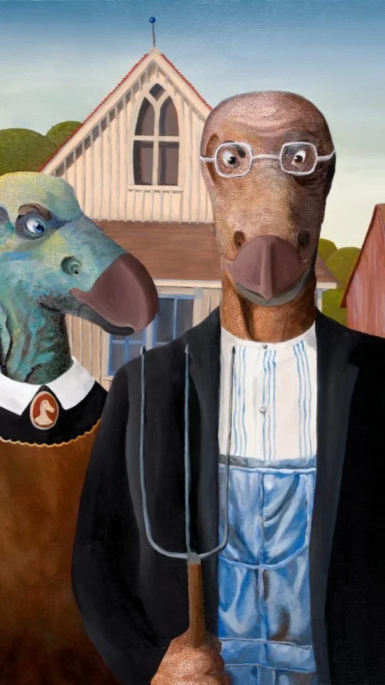
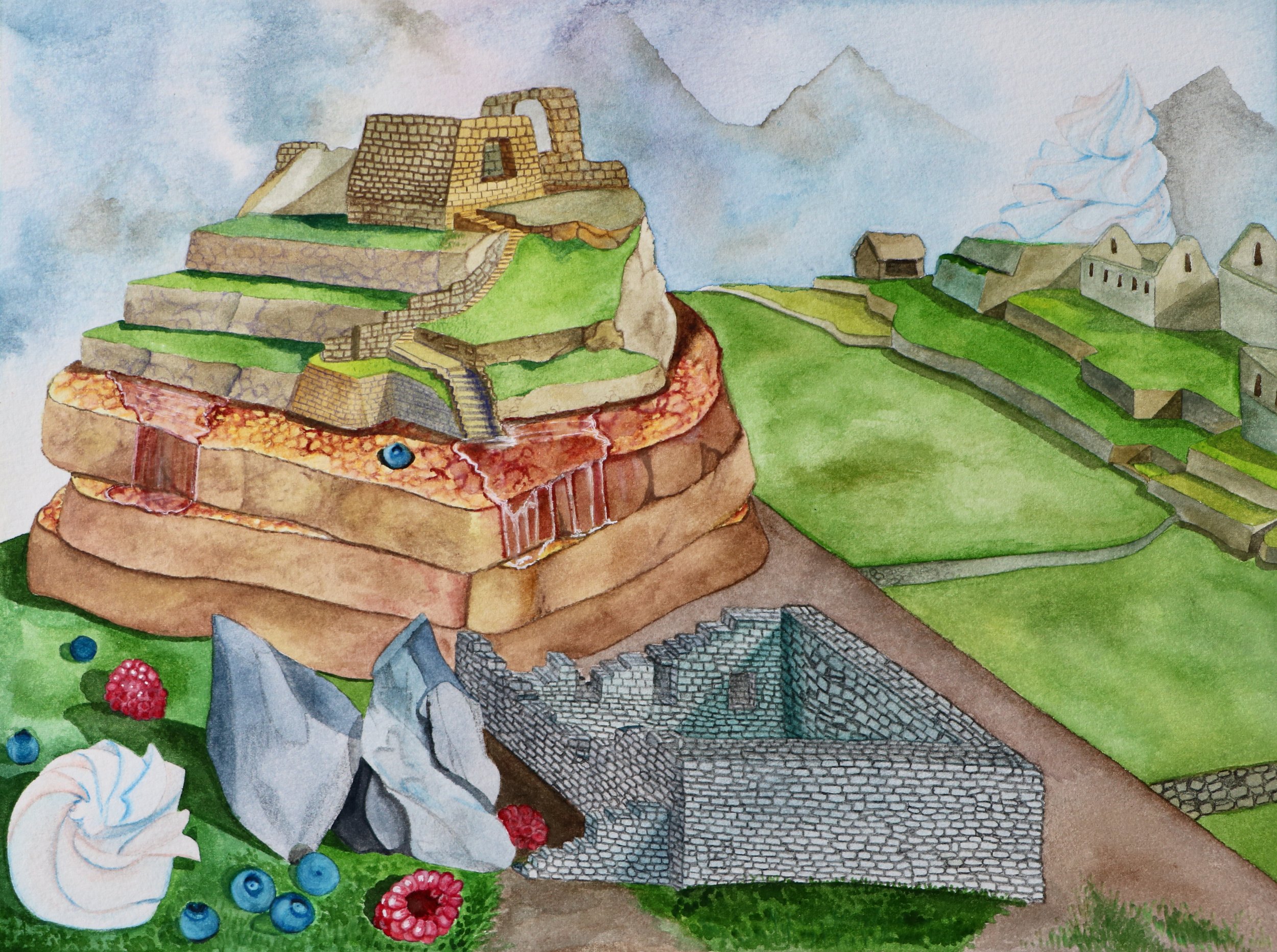
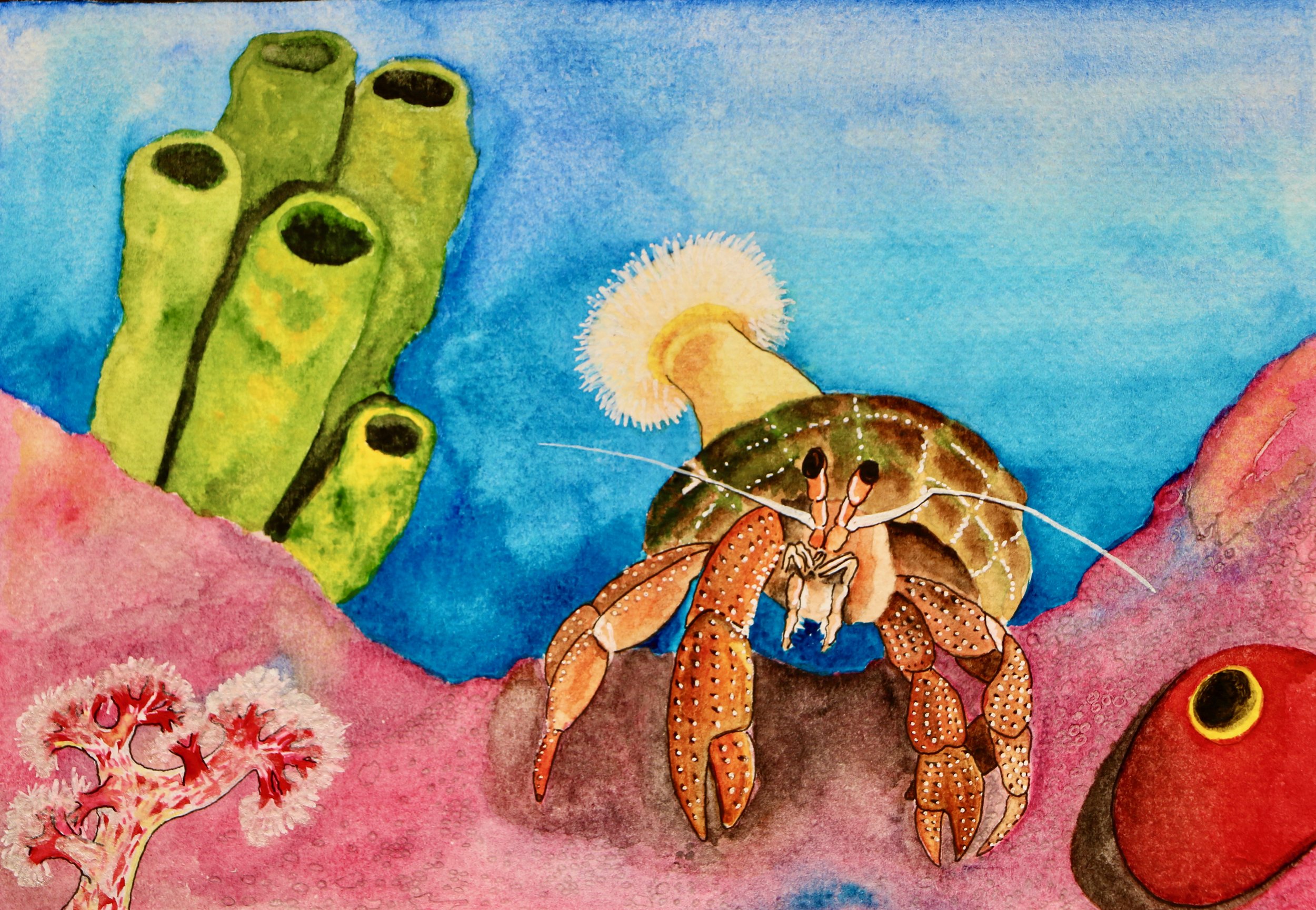
Next I've tried one of my Unstill Life paintings:

In [13]:
def what_is_it(filename):
image = PIL.Image.open(filename)
image_array = np.array(image)[np.newaxis, :, :, 0:3]
prediction = sess.run(output_tensor, {'input:0': image_array})
prediction = prediction.max(axis=0)
top_pred = prediction.argsort()[-5:][::-1]
for i in range(5):print(i+1, ' ', lines[top_pred[i]].strip('\n'), ' ', int(prediction[top_pred[i]]*100), '% \n')
return
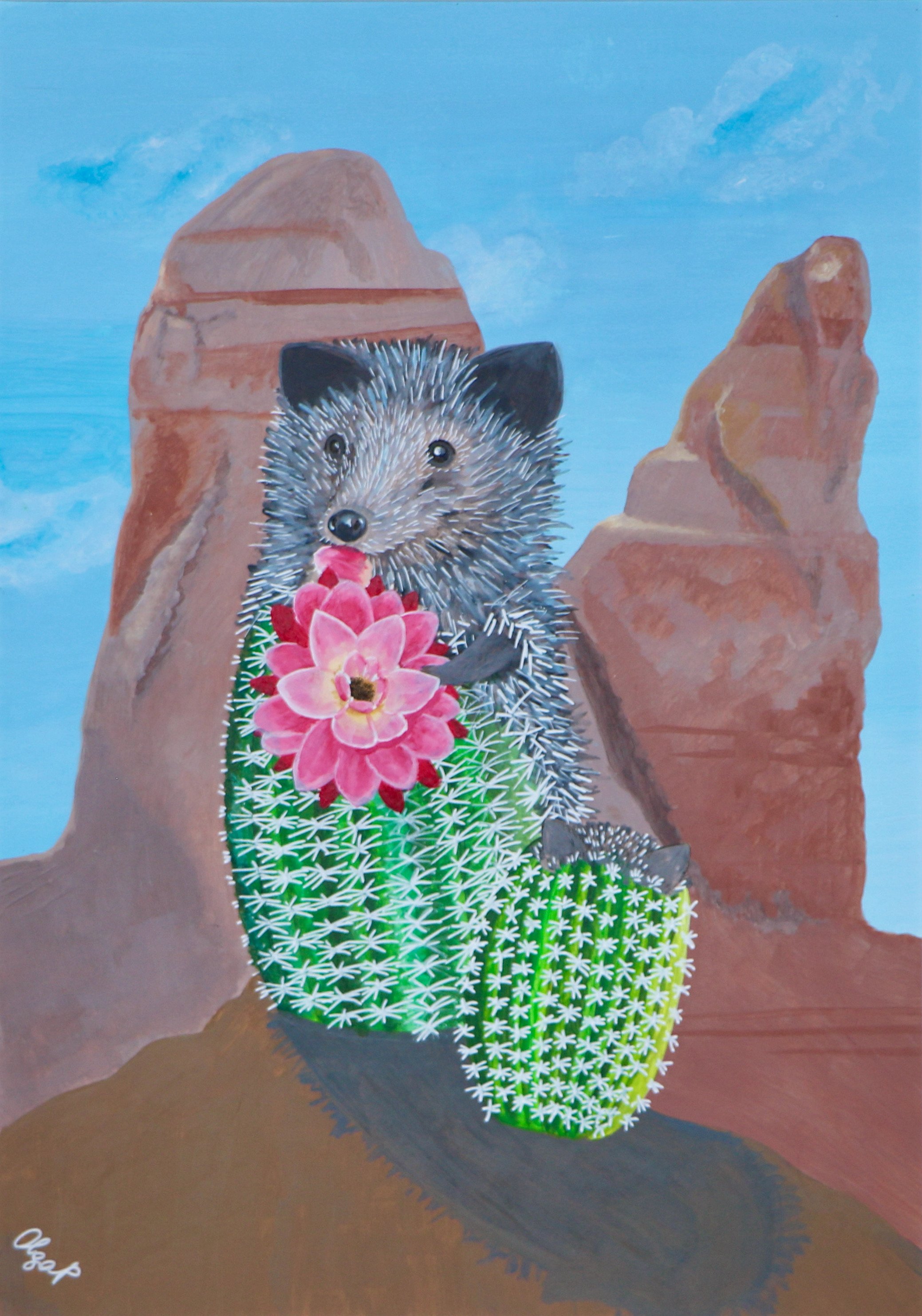
what_is_it("deserthedgehog.jpg")
Out:
1 quill 88 %
2 volcano 84 %
3 cliff 66 %
4 porcupine 60 %
5 sarong 48 %
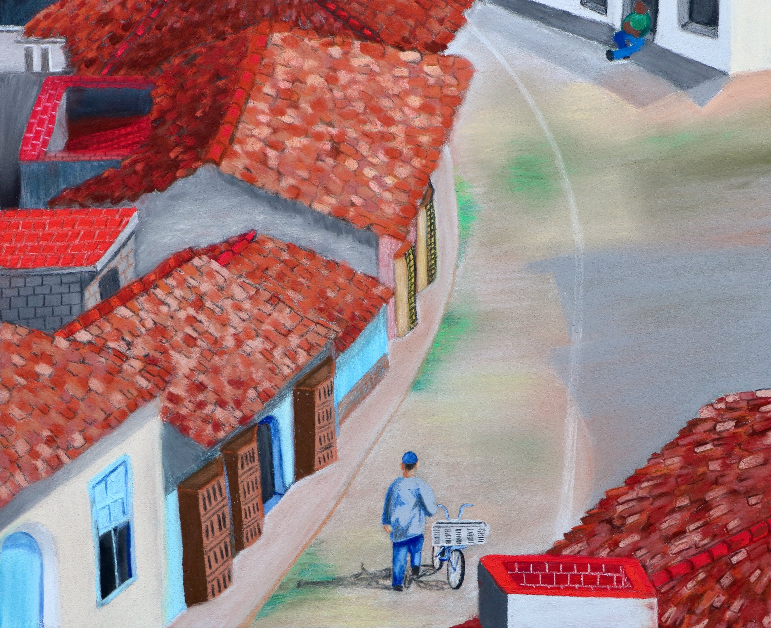
Quill, seriously? Okay, maybe it's the shadow. But I can see how it could get the others. Lets try cropping different areas of the painting and run the Inception on them:

In [14]:
what_is_it("hedgecrop1.jpg")
what_is_it("hedgecrop2.jpg")
Out:
1 pot 84 %
2 chainlink fence 20 %
3 tray 4 %
4 vase 3 %
5 strawberry 2 %
1 hamster 46 %
2 porcupine 36 %
3 beaver 16 %
4 otter 4 %
5 mousetrap 2 %
Again, I see how these could come about. I am a little hurt that Inception found my Mme Hedgehog to look more like a hamster than a porcupine (not to mention, not at all like a hedgehog), but I can live with that.
In [15]:
sess.close()
Shop original artworks from the Studio Sale:


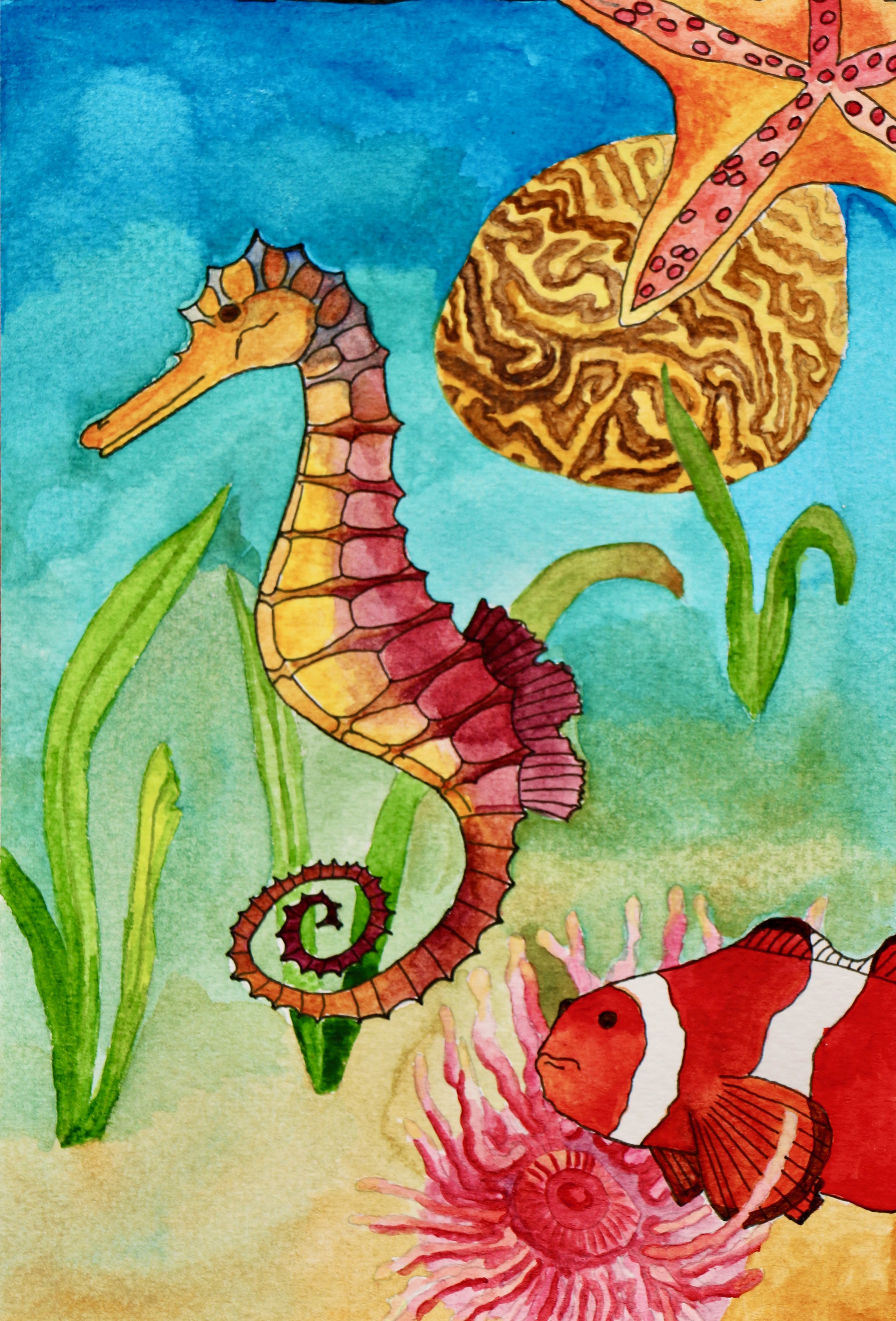
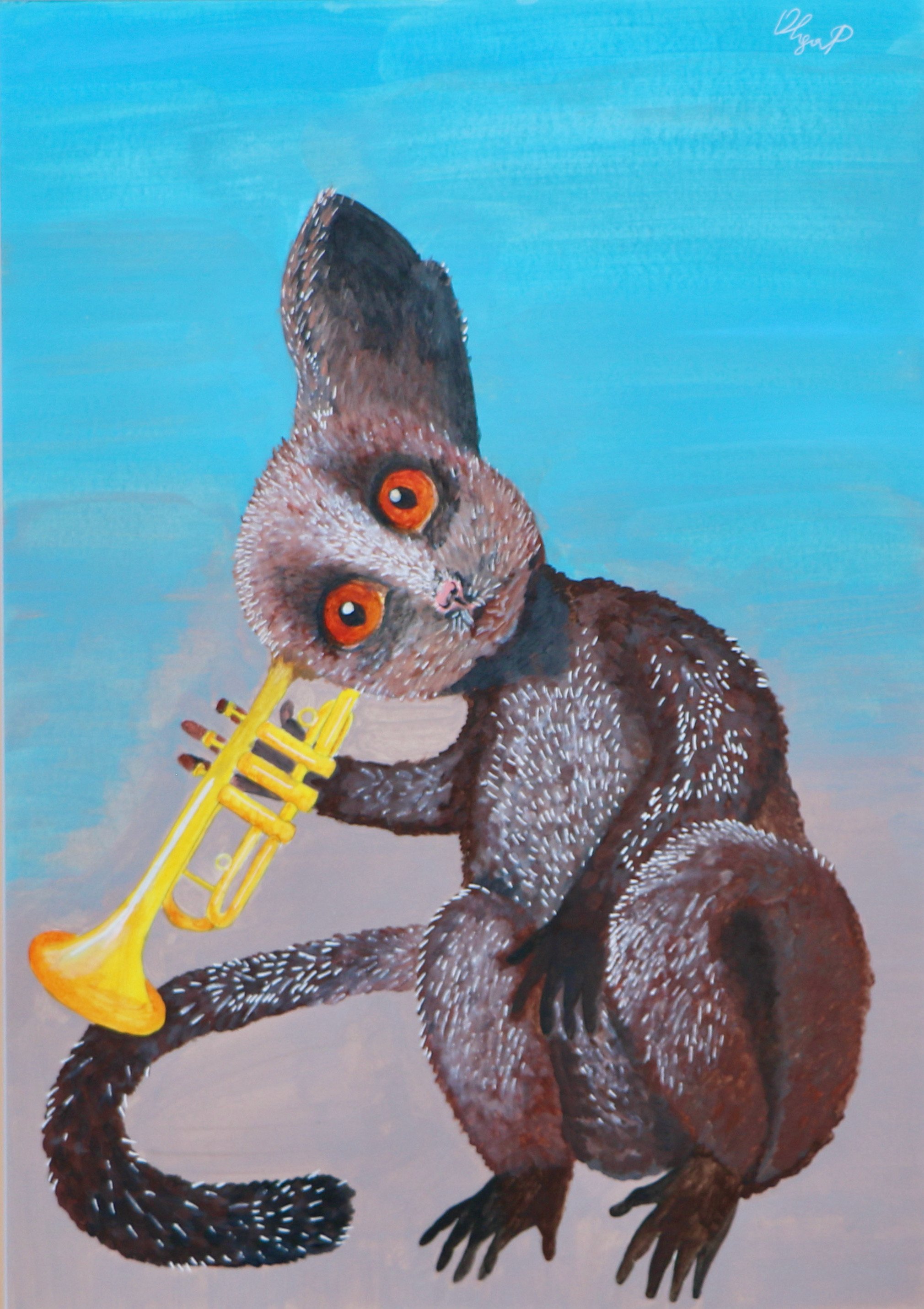
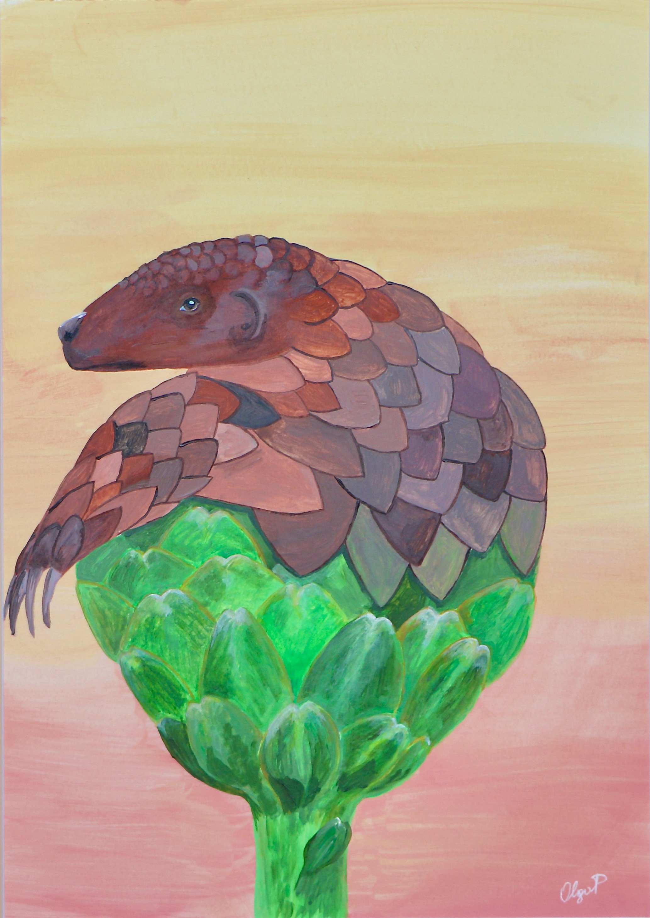
The latest work in progress from instagram.com/olgapaints: